Polyphase and NPR Filter Bank with Chirp Functions
This example shows the result of near perfect reconstruction (NPR) and standard polyphase filter banks on channelizing a chirp signal.
[1]:
from pathlib import Path
import numpy as np
import scipy.signal as sig
from mitarspysigproc import (
    pfb_decompose,
    pfb_reconstruct,
    kaiser_coeffs,
    kaiser_syn_coeffs,
    npr_analysis,
    npr_synthesis,
    rref_coef,
)
import matplotlib.pyplot as plt
[2]:
def create_chirp(t_len, fs, bw, pad, nchans, nslice):
"""Creates a chirp signal
Parameters
----------
t_len : float
Length of chirp in seconds
fs : float
Sampling frequency in Hz
bw : float
Bandwidth of chirp
nzeros : tuple
Number of zeros to pad in the begining and end of the array.
nchans : int
Number of channels for the PFB
nslice : int
Number of time samples from the pfb
Returns
-------
tout : ndarray
The time vector for the created signal
xout : ndarray
Created signal
"""
nar = (
np.arange(int(-nslice * nchans / 2), int(nslice * nchans / 2), dtype=float)
/ nslice
/ nchans
)
t = np.linspace(-t_len / 2, t_len / 2, int(t_len * fs))
dphi = 2 * np.pi * nar * bw / fs
phi = np.mod(np.cumsum(dphi), 2 * np.pi)
x = np.exp(-1j * phi)
# x = sig.chirp(t,t1=t_len,f0=0,f1=bw,method='linear')
xout = np.concatenate((pad[0], x, pad[1]), axis=0)
tp1 = -1 * np.arange(0, len(pad[0]), dtype=float)[::-1] / fs - t_len / 2
tp2 = np.arange(0, len(pad[1]), dtype=float) / fs + t_len / 2
tout = np.concatenate((tp1, t, tp2), axis=0)
return tout, xout
def runchirptest(t_len, fs, bw, nzeros, nchans, nslice):
"""Creates a chirp and runs the standard PFB analysis and reconstruction
Parameters
----------
t_len : float
Length of chirp in seconds
fs : float
Sampling frequency in Hz
bw : float
Bandwidth of chirp
nzeros : int
Number of zeros to pad
nchans : int
Number of channels for the PFB
nslice : int
Number of time samples from the pfb
Returns
-------
x_rec : ndarray
Reconstructed signal
tin : ndarray
The time vector for the input signal
x : ndarray
Input signal
x_pfb : ndarray
The result of the PFB analysis in an nchans x slice array.
"""
pad = [np.zeros(nzeros), np.zeros(nzeros)]
t, x = create_chirp(t_len, fs, bw, pad, nchans, nslice)
coeffs = kaiser_coeffs(nchans, 8.0)
mask = np.ones(nchans, dtype=bool)
xout = pfb_decompose(x, nchans, coeffs, mask)
fillmethod = ""
fillparams = [0, 0]
syn_coeffs = kaiser_syn_coeffs(nchans, 8)
x_rec = pfb_reconstruct(
xout, nchans, syn_coeffs, mask, fillmethod, fillparams=[], realout=False
)
return x_rec, t, x, xout
def runnprchirptest(t_len, fs, bw, nzeros, nchans, nslice, ntaps=64):
"""Creates a chirp and runs the near perfect PFB analysis and reconstruction
Parameters
----------
t_len : float
Length of chirp in seconds
fs : float
Sampling frequency in Hz
bw : float
Bandwidth of chirp
nchans : int
Number of channels for the PFB
nslice : int
Number of time samples from the pfb
Returns
-------
x_rec : ndarray
Reconstructed signal
tin : ndarray
The time vector for the input signal
x : ndarray
Input signal
x_pfb : ndarray
The result of the PFB analysis in an nchans x slice array.
"""
pad = [np.zeros(nzeros), np.zeros(nzeros)]
t, x = create_chirp(t_len, fs, bw, pad, nchans, nslice)
coeffs = rref_coef(nchans, ntaps)
mask = np.ones(nchans, dtype=bool)
xout = npr_analysis(x, nchans, coeffs)
fillmethod = ""
fillparams = [0, 0]
x_rec = npr_synthesis(xout, nchans, coeffs)
return x_rec, t, x, xout
def nexpow2(x):
"""Returns the next power of two.
Parameters
----------
x : int
Inital number.
Returns
-------
int
The next power of two of x.
"""
return int(np.power(2, np.ceil(np.log2(x))))
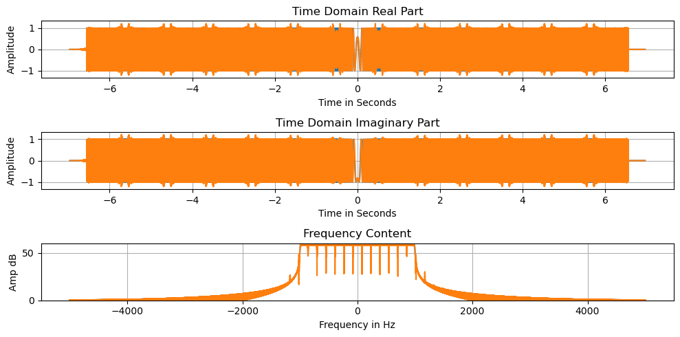
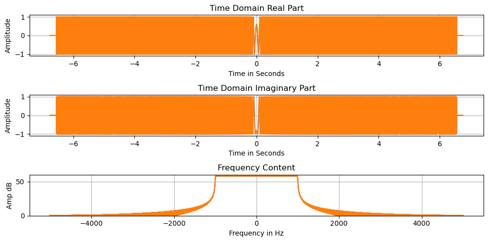
def plotdata(x, x_rec, tin, tout, g_del=0):
"""Plot the data and return the figure.
Parameters
----------
x : ndarray
Input signal
x_rec : ndarray
Reconstructed signal
tin : ndarray
The time vector for the input signal
tout : ndarray
The time vector for the output signal
Returns
-------
fig : matplotlib.fig
The matplotlib fig for plotting or saving.
"""
fig, ax = plt.subplots(3, 1, figsize=(10, 5))
inlen = x.shape[0]
outlen = x_rec.shape[0]
tau = tin[1] - tin[0]
ax[0].plot(tin, x.real, label="Input")
ax[0].plot(tout, np.roll(x_rec.real, -g_del), label="Output")
ax[0].set_xlabel("Time in Seconds")
ax[0].set_ylabel("Amplitude")
ax[0].set_title("Time Domain Real Part")
ax[0].grid(True)
ax[1].plot(tin, x.imag, label="Input")
ax[1].plot(tout, np.roll(x_rec.imag, -g_del), label="Output")
ax[1].set_xlabel("Time in Seconds")
ax[1].set_ylabel("Amplitude")
ax[1].set_title("Time Domain Imaginary Part")
ax[1].grid(True)
nfft_in = nexpow2(inlen)
nfft_out = nexpow2(outlen)
in_freq = np.fft.fftshift(np.fft.fftfreq(nfft_in, d=tau))
out_freq = np.fft.fftshift(np.fft.fftfreq(nfft_out, d=tau))
spec_in = np.abs(np.fft.fftshift(np.fft.fft(x, n=nfft_in))) ** 2
spec_out = np.abs(np.fft.fftshift(np.fft.fft(x_rec[:, 0], n=nfft_out))) ** 2
spec_in_log = 10 * np.log10(spec_in)
spec_out_log = 10 * np.log10(spec_out)
ax[2].plot(in_freq, spec_in_log, label="Input")
ax[2].plot(out_freq, spec_out_log, label="Output")
ax[2].set_xlabel("Frequency in Hz")
ax[2].set_ylabel("Amp dB")
ax[2].set_title("Frequency Content")
ax[2].grid(True)
ax[2].set_ylim([0, 60])
fig.tight_layout()
return fig
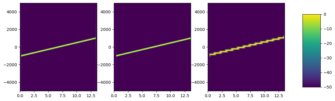
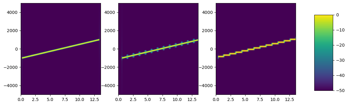
def plot_spectrogram(x, x_rec, x_pfb):
"""Plots the input signal, pfb output and reconstructed signal.
Parameters
----------
x : ndarray
Input signal
x_rec : ndarray
Reconstructed signal
x_pfb : ndarray
The result of the PFB analysis in an nchans x slice array.
Returns
-------
fig : matplotlib.fig
The matplotlib fig for plotting or saving.
"""
fig, ax = plt.subplots(1, 3, figsize=(12, 3.5))
nfft = 256
w = sig.get_window("blackman", nfft)
SFT = sig.ShortTimeFFT(
w, hop=nfft, fs=10000, mfft=nfft, scale_to="magnitude", fft_mode="centered"
)
sxin = 20 * np.log10(np.abs((SFT.stft(x))) + 1e-12)
sxout = 20 * np.log10(np.abs((SFT.stft(x_rec))) + 1e-12)
im1 = ax[0].imshow(
sxin[::-1],
origin="lower",
aspect="auto",
extent=SFT.extent(len(x)),
cmap="viridis",
vmin=-50,
vmax=0,
)
im2 = ax[1].imshow(
sxout[::-1],
origin="lower",
aspect="auto",
extent=SFT.extent(len(x_rec)),
cmap="viridis",
vmin=-50,
vmax=0,
)
nchan, nslice = x_pfb.shape
x_pfb = np.fft.fftshift(x_pfb / np.abs(x_pfb.flatten()).max(), axes=0)
x_pfb_db = 20 * np.log10(np.abs(x_pfb) + 1e-12)
im3 = ax[2].imshow(
x_pfb_db,
origin="lower",
aspect="auto",
extent=SFT.extent(len(x_rec)),
cmap="viridis",
vmin=-50,
vmax=0,
)
fig.tight_layout()
fig.subplots_adjust(right=0.8)
cbar_ax = fig.add_axes([0.85, 0.15, 0.05, 0.7])
fig.colorbar(im3, cax=cbar_ax)
return fig
[3]:
nchans = 64
nslice = 2048
fs = 10000
t_len = nchans * nslice / fs
bw = 2000
ntaps = 64
g_del = nchans * (ntaps - 1) // 2
nzeros = 2048

x_rec, t, x, xpfb = runchirptest(t_len, fs, bw, nzeros*2, nchans, nslice)
# x_rec = x_rec[:len(x)]

fig = plotdata(x, x_rec[:t.shape[0],:], t, t,nchans*ntaps)
[11]:
fig2 = plot_spectrogram(x, x_rec[:, 0], xpfb[:, :, 0])
[23]:
x_rec, t, x, xpfb = runnprchirptest(t_len, fs, bw, nzeros, nchans, nslice, ntaps)
x_rec = x_rec[: len(x), np.newaxis]  # need to add new axis due to plotting issue

fig = plotdata(x, x_rec, t, t, g_del)

print(x.shape)
print(x_rec.shape)
print(t.shape)
(135168,)
(135168, 1)
(135168,)
[24]:
fig2 = plot_spectrogram(x, x_rec[:, 0], xpfb)